Imágenes con frases de Amor y Amistad para compartir, bonitas tarjetas virtuales de amor para el Día de San Valentín 2024, mejores Imágenes de Feliz Año Nuevo 2025 para compartir, Frases bonitas para felicitar en Navidad, cada día agregamos nuevas frases de amor cortas y bonitas para que puedas dedicar a tu pareja o seres queridos, imágenes con frases cortas de amor originales para que puedas enviar a través de Facebook, WhatsApp, Instagram o Twitter, descubre aquí todos los días la frases más lindas de amor con mensajes muy bonitos para regalar o dedicar, cada una de estas imágenes son totalmente gratuitas y puedes descargar para que puedas enviar a tus seres amados.


Últimos imágenes con Frases de amor y Amistad
En esta sección publicamos nuevas imágenes con frases cortos de amor y amistad para que puedas dedicar con mucho cariño a tu pareja.


Últimos imágenes con Frases de Navidad y Año Nuevo 2025
En esta sección publicamos últimos imágenes y frases cortos de Navidad 2023 y Año Nuevo 2024, cada una de estas bonitas imágenes navidad puedes descargar para luego compartir a través de diferentes redes sociales